Supervised patch detection
patch_detection.Rd![[Experimental]](figures/lifecycle-experimental.svg)
A patch is defined as a subgraph which is enriched for a set of patch-specific protein markers. A patch should typically have a different origin than the bulk of the PNA graph. A typical example of a patch is a small piece of another cell, e.g. a patch of a B cell on a T cell (receiver).
This analysis tool requires a predefined set of patch-specific protein markers and is therefore
a supervised method. Patch-specific means that these markers are high abundant on the patch
and low abundant on the receiver cell. Optimal patch markers are those that are high abundant
and highly specific. The method is sensitive to the choice of patch markers and therefore
requires careful selection. See identify_markers_for_patch_analysis for more
information on how to select patch markers.
Patch detection can be used to find multiple patches in a single PNA graph. These subgraphs can be leveraged to study the patch protein composition, patch proximity scores, number of patches and the fraction of the receiver cell covered by patches. Note that patches can appear from cell debris or from artificial bleedover and doesn't necessarily indicate a cell-cell interaction. If you aim to study patch composition in response to a specific treatment or condition, it is recommended to include a control population for reference.
Two algorithms are available for patch detection, described in the sections below.
Usage
patch_detection(
  cg,
  patch_markers,
  receiver_markers = NULL,
  k = 2L,
  leiden_resolution = 0.005,
  patch_nodes_threshold = 100,
  prune_patch_edge = TRUE,
  leiden_refinement = TRUE,
  method = c("expand_contract", "local_G"),
  contraction = 0.5,
  pval_threshold = 0.01,
  seed = 123,
  verbose = TRUE
)
Arguments
- cg
A
CellGraphobject with PNA data.- patch_markers
A character vector with the names of the markers that are exclusively found on the patches, e.g. "CD41" for platelets.
- receiver_markers
An optional character vector with the names of the markers that are exclusively found on the receiver cell.
- k
The number of nearest neighbors to consider for the expansion or for local G.
- leiden_resolution
The resolution parameter for the Leiden algorithm.
- patch_nodes_threshold
The minimum number of nodes to consider a patch.
- prune_patch_edge
A logical indicating if edge nodes of the patches should be pruned.
- leiden_refinement
A logical indicating if the patch graph should be refined into smaller communities using Leiden. This is useful if there are weakly connected patches.
- method
A character indicating the method to use for patch detection. Must be one of "expand_contract" or "local_g".
- contraction
A numeric value between 0 and 1 that controls the number of nodes to keep in the "expand_contract" method. Higher values will increase contraction and result in smaller patches.
- pval_threshold
A numeric value that controls the p value threshold for the "local_g" method.
- seed
Set seed for reproducibility
- verbose
A logical indicating if messages should be printed to the console.
Value
A CellGraph object with two additional node columns in the tbl_graph object:
patch: An integer vector indicating the patch each node belongs to.potential_patch: An integer vector indicating potential patches which are smaller thanpatch_nodes_threshold.
Expand and contract
Initialization: Start with the set of nodes
Plabelled by patch-specific protein markers.Expansion:
Expand
Pto include nodes that connect with at least 2 nodes inPwithin ak-step neighborhood.Expand
Pto include nodes that connect with at least 2 nodes inPwithin a 1-step neighborhood.
Contract
Pby only keeping nodes with the highest in- out-degree ratio. The number of kept nodes is controlled by thecontractionparameter.(optional) Remove nodes from
Pat the patch border with low patch connectivityConstruct the patch graph from
P, split it into its connected components and remove components smaller thanpatch_nodes_threshold(optional) Run community detection (Leiden) to split up weakly connected patch components and repeat the
patch_nodes_thresholdfiltering step. Theleiden_resolutionparameter controls the granularity of the communities, where a higher value is more likely to result in more patches and vice versa.Label nodes in the original graph with the patch information. The largest "patch" is labeled as 0 and should correspond to the receiver cell graph. The rest of the patches are labeled as 1, 2, etc. and correspond to patches ordered by decreasing size.
Local G
Run local G using the
patch_markersUMI counts.Define
Pas the set of nodes with a p value for the local G Z score belowpval_threshold.(optional) Remove nodes from
Pat the patch border with low patch connectivityConstruct the patch graph from
P, split it into its connected components and remove components smaller thanpatch_nodes_threshold.(optional) Run community detection (Leiden) to split up weakly connected patch components and repeat the
patch_nodes_thresholdfiltering step. Theleiden_resolutionparameter controls the granularity of the communities, where a higher value is more likely to result in more patches and vice versa.Label nodes in the original graph with the patch information. The largest "patch" is labeled as 0 and should correspond to the receiver cell graph. The rest of the patches are labeled as 1, 2, etc. and correspond to patches ordered by decreasing size.
Examples
library(tidygraph)
library(dplyr)
library(ggplot2)
library(Matrix)
# Load a CellGraph object with PNA data
se <- ReadPNA_Seurat(minimal_pna_pxl_file()) %>%
LoadCellGraphs(cells = colnames(.)[1], add_layouts = TRUE)
#> ✔ Created a <Seurat> object with 5 cells and 158 targeted surface proteins
#> ℹ Fetching edgelists for 1 cells
#> → Creating <CellGraph> objects
#> → Fetching marker counts
#> → Adding marker counts to <CellGraph> object(s)
#> → Fetching layouts
#> → Adding layouts to <CellGraph> object(s)
#> ✔ Successfully loaded 1 <CellGraph> object(s).
cg <- CellGraphs(se)[[1]]
protein_props <- cg@counts %>%
Matrix::colSums() %>%
prop.table()
patch_props <- protein_props
patch_props["CD8"] <- 0.4
patch_props <- patch_props %>% prop.table()
# Here we'll create an artifical patch by replacing node counts
# in a small region
inds <- 1
patch_size <- 1000
xyz <- cg@layout$wpmds_3d %>% as.matrix()
xyz_center <- xyz[inds, , drop = FALSE]
dists <- 1 - cos_dist(A = xyz_center, B = xyz) %>% as.vector()
inds_replace <- order(dists)[1:patch_size]
counts_with_patch <- cg@counts
# Create a count matrix for the patch
# enriched for CD8
j <-
sample(
x = seq_len(length(patch_props)),
size = length(inds_replace),
prob = patch_props,
replace = TRUE
)
i <- seq_len(length(inds_replace))
x <- rep(1, length(i))
dims <- c(length(inds_replace), length(patch_props))
dimnames <- list(rownames(counts_with_patch)[inds_replace], names(patch_props))
counts <- Matrix::sparseMatrix(
i = i,
j = j,
x = x,
dims = dims,
dimnames = dimnames
)
counts_with_patch[inds_replace, ] <- counts
cg@counts <- counts_with_patch
# Run patch detection
cg <- patch_detection(
cg,
patch_markers = "CD8"
)
#> ℹ Extracting connected patches using method "expand_contract"...
#> Warning: 'as(<dgCMatrix>, "ngCMatrix")' is deprecated.
#> Use 'as(., "nMatrix")' instead.
#> See help("Deprecated") and help("Matrix-deprecated").
#> → 1592 out of 43543 nodes are labelled as patch nodes...
#> → Found 1 connected patches after filtering...
#> → Splitting up weakly connected patches using Leiden with resolution=0.005...
#> ℹ Found 1 patches after splitting...
#> ✔ Finished!
# Visualize patch
xyz <- cg@layout$wpmds_3d %>%
mutate(patch = cg@cellgraph %>% pull(patch))
plotly::plot_ly(
xyz,
x = ~x, y = ~y, z = ~z,
color = ~ factor(patch),
type = "scatter3d",
mode = "markers",
colors = c("lightgrey", "red"),
marker = list(
size = 2
)
)
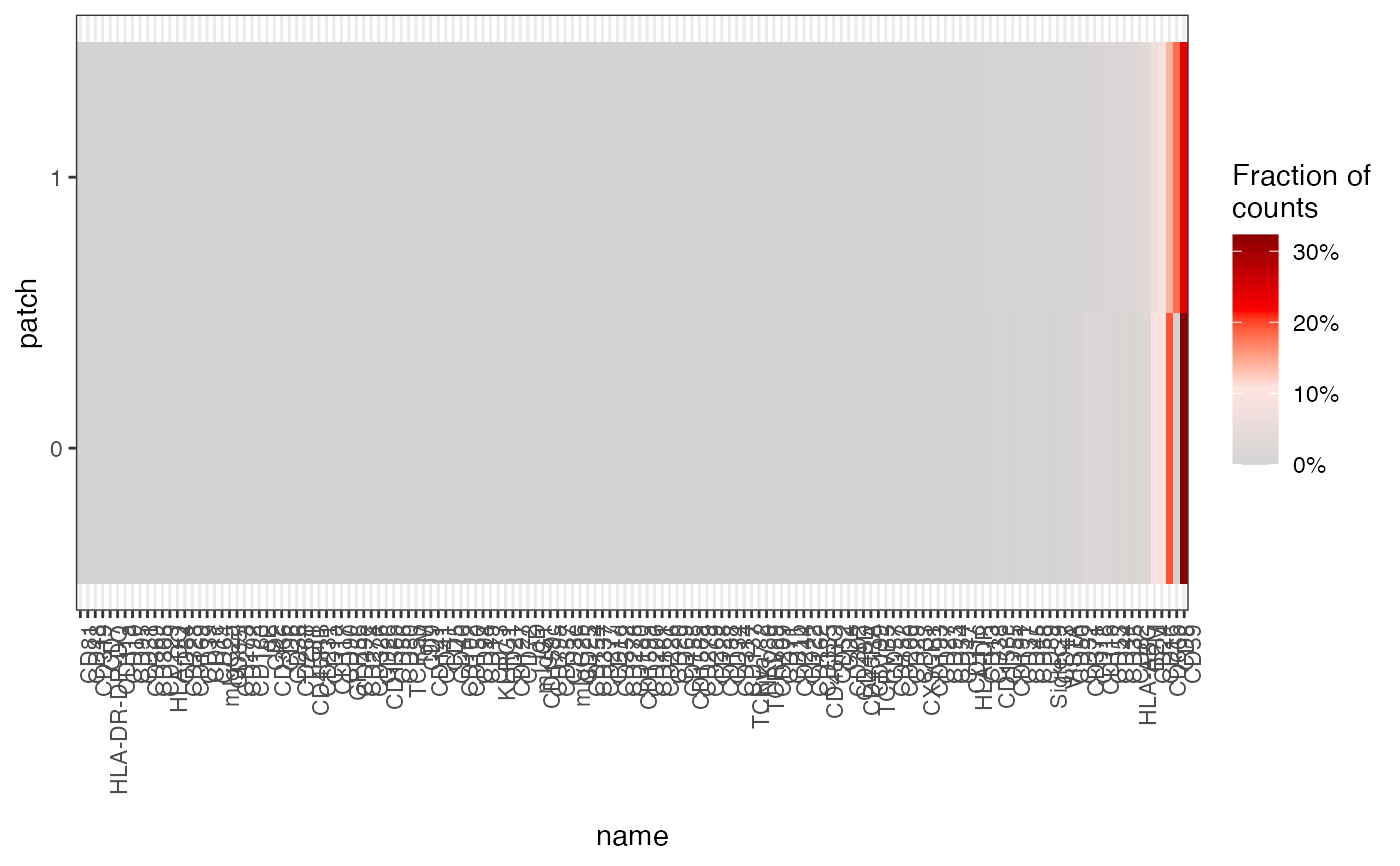
# Check protein composition
gg <- tibble(patch = cg@cellgraph %>% pull(patch) %>% as.factor()) %>%
bind_cols(as.matrix(cg@counts)) %>%
group_by(patch) %>%
summarize(across(where(is.numeric), ~ sum(.x))) %>%
tidyr::pivot_longer(where(is.numeric)) %>%
group_by(patch) %>%
mutate(value = value / sum(value))
lvls <- gg %>%
arrange(desc(patch), value) %>%
pull(name) %>%
unique()
ggplot(gg %>% mutate(name = factor(name, lvls)), aes(name, patch, fill = value)) +
geom_tile() +
scale_fill_gradientn(
colours = c("lightgrey", "mistyrose", "red", "darkred"),
label = scales::percent
) +
theme_bw() +
theme(axis.text.x = element_text(angle = 90, hjust = 1)) +
labs(fill = "Fraction of\ncounts")