Load data
2023-12-18
load_data.RmdTip: you can turn off the verbose messages in pixelatorR
by setting:
options(pixelatorR.verbose = FALSE)In this tutorial, we will take a closer look at the functions provided in
pixelatorRto load data. This is mainly intended for advanced users. If you want to learn more about how to analyze MPX/PNA data, please visit our tutorials.
Load data
To get started, we need a PXL file which we can download from https://software.pixelgen.com/.
dir.create("PBMC_data")
download.file(url = "https://pixelgen-technologies-datasets.s3.eu-north-1.amazonaws.com/mpx-datasets/pixelator/0.12.0/1k-human-pbmcs-v1.0-immunology-I/Sample01_human_pbmcs_unstimulated.dataset.pxl?download=1",
              destfile = "PBMC_data/Sample01_human_pbmcs_unstimulated.dataset.pxl")
pixelatorR provides several functions to load data from
a PXL file.
For instance, ReadMPX_counts allows us to load only the
count matrix and nothing else:
pxl_file <- "PBMC_data/Sample01_human_pbmcs_unstimulated.dataset.pxl"
countMatrix <- ReadMPX_counts(pxl_file)
countMatrix[1:5, 1:5]
## RCVCMP0000000 RCVCMP0000002 RCVCMP0000003 RCVCMP0000005 RCVCMP0000006
## CD274 62 11 25 31 16
## CD44 553 180 66 347 213
## CD25 12 7 6 8 5
## CD279 4 2 0 8 2
## CD41 6 1 3 5 6With ReadMPX_item, we can chose a specific item to load
from the PXL file, including: “polarization”, “colocalization”,
“edgelist”.
polarization_scores <- ReadMPX_item(pxl_file, items = "polarization")
polarization_scores
## # A tibble: 33,479 × 6
## morans_i morans_p_value morans_p_adjusted morans_z marker component
## <dbl> <dbl> <dbl> <dbl> <chr> <chr>
## 1 -0.00299 0.772 1.000 -0.290 ACTB RCVCMP0000830
## 2 -0.0161 0.177 0.771 -1.35 B2M RCVCMP0000830
## 3 0.0147 0.125 0.633 1.53 CD102 RCVCMP0000830
## 4 -0.00678 0.590 1.000 -0.539 CD11a RCVCMP0000830
## 5 0.000836 0.891 1.000 0.137 CD127 RCVCMP0000830
## 6 -0.00132 0.145 0.693 -1.46 CD150 RCVCMP0000830
## 7 -0.00103 0.395 1.000 -0.851 CD152 RCVCMP0000830
## 8 -0.00162 0.0365 0.265 -2.09 CD154 RCVCMP0000830
## 9 -0.000919 0.971 1.000 -0.0364 CD162 RCVCMP0000830
## 10 -0.000345 0.561 1.000 0.582 CD163 RCVCMP0000830
## # ℹ 33,469 more rowsIf we provide multiple items, ReadMPX_item returns a
list instead:
all_items <- ReadMPX_item(pxl_file, items = c("polarization", "colocalization", "edgelist"))
names(all_items)
## [1] "polarization" "colocalization" "edgelist"Alternatively, we can use the wrapper functions
ReadMPX_polarization, ReadMPX_colocaliztion
and ReadMPX_edgelist to do the same thing as
ReadMPX_item:
polarization_scores <- ReadMPX_polarization(pxl_file)is equivalent to
polarization_scores <- ReadMPX_item(pxl_file, items = "polarization")Seurat
Perhaps the most useful function here is ReadMPX_Seurat
which allows us to load MPX data into a Seurat object with
some additional bells and whistles provided by
pixelatorR.
seur_obj <- ReadMPX_Seurat(pxl_file)## ! Failed to remove temporary file C:/Users/max/AppData/Local/Temp/RtmpEJyw2L/file5bc84dc0555.h5adHere, you have a few options to modify how the Seurat
should be created. First and foremost, we can set
return_cellgraphassay = FALSE to return a
Seurat object which only includes abundance
measurements.
In this simpler data set, only the count matrix is stored as an
Assay without any spatial data. This means that almost all
information that is unique to MPX will be ignored so you will not be
able to analyze or visualize graphs and there will be no way to explore
the spatial statistics.
However, this basic data set uses significantly less memory and is faster to process which can be useful if protein abundance is the only interesting data type for the analysis.
# Load simpler data set
seur_obj <- ReadMPX_Seurat(pxl_file, return_cellgraphassay = FALSE)
## Warning: Data is of class matrix. Coercing to dgCMatrix.## ! Failed to remove temporary file C:/Users/max/AppData/Local/Temp/RtmpEJyw2L/file5bc872e246ec.h5ad
seur_obj[["mpxCells"]]## Assay (v5) data with 80 features for 477 cells
## Top 10 variable features:
## CD274, CD44, CD25, CD279, CD41, HLA-ABC, CD54, CD26, CD27, CD38
## Layers:
## countsBy default, ReadMPX_Seurat returns the MPX data in an
object called CellGraphAssay. This object class extends the
Assay class from Seurat and is essentially an
Assay object with additional data slots. The
CellGraphAssay class will be covered in more detail later
in this tutorial.
Most additional parameters in ReadMPX_Seurat controls
the behavior when return_cellgraphassay = TRUE. By default,
the MPX polarization scores and colocalization scores are loaded and
stored in a CellGraphAssay named “mpxCells”.
seur_obj <- ReadMPX_Seurat(pxl_file)## ! Failed to remove temporary file C:/Users/max/AppData/Local/Temp/RtmpEJyw2L/file5bc86f5e21d7.h5ad
seur_obj## An object of class Seurat
## 80 features across 477 samples within 1 assay
## Active assay: mpxCells (80 features, 80 variable features)
## 1 layer present: countsSpatial metrics
We can fetch the polarization/colocalization score tables from the
Seurat object with the PolarizationScores and
ColocalizationScores methods:
# Fetch polarization scores
polarizaton_scores <- PolarizationScores(seur_obj)
polarizaton_scores %>% head()
## # A tibble: 6 × 6
## morans_i morans_p_value morans_p_adjusted morans_z marker component
## <dbl> <dbl> <dbl> <dbl> <chr> <chr>
## 1 -0.00299 0.772 1.000 -0.290 ACTB RCVCMP0000830
## 2 -0.0161 0.177 0.771 -1.35 B2M RCVCMP0000830
## 3 0.0147 0.125 0.633 1.53 CD102 RCVCMP0000830
## 4 -0.00678 0.590 1.000 -0.539 CD11a RCVCMP0000830
## 5 0.000836 0.891 1.000 0.137 CD127 RCVCMP0000830
## 6 -0.00132 0.145 0.693 -1.46 CD150 RCVCMP0000830
# Fetch colocalization scores
colocalization_scores <- ColocalizationScores(seur_obj)
colocalization_scores %>% head()
## # A tibble: 6 × 15
## marker_1 marker_2 pearson pearson_mean pearson_stdev pearson_z pearson_p_value
## <chr> <chr> <dbl> <dbl> <dbl> <dbl> <dbl>
## 1 ACTB ACTB 1 1 0 NA NA
## 2 ACTB B2M 0.324 0.317 0.0162 0.429 0.334
## 3 B2M B2M 1 1 0 NA NA
## 4 ACTB CD102 0.304 0.235 0.0167 4.17 0.0000151
## 5 B2M CD102 0.604 0.614 0.00966 -1.06 0.145
## 6 CD102 CD102 1 1 0 NA NA
## # ℹ 8 more variables: pearson_p_value_adjusted <dbl>, jaccard <dbl>,
## # jaccard_mean <dbl>, jaccard_stdev <dbl>, jaccard_z <dbl>,
## # jaccard_p_value <dbl>, jaccard_p_value_adjusted <dbl>, component <chr>An equivalent way to extract the polarization scores would be:
polarizaton_scores <- seur_obj[["mpxCells"]]@polarizationBut it’s good practice to use
PolarizationScores/ColocalizationScores which
is easier to read. One just have to make sure that the
DefaultAssay is set to “mpxCells”.
QC metrics
Component-specific metrics are stored in the @meta.data
slot of the Seurat object which can be accessed with double
brackets ([[]]):
colnames(seur_obj[[]])## [1] "antibodies" "edges" "leiden"
## [4] "mean_reads" "mean_umi_per_upia" "mean_upia_degree"
## [7] "median_reads" "median_umi_per_upia" "median_upia_degree"
## [10] "reads" "tau" "tau_type"
## [13] "umi" "umi_per_upia" "upia"
## [16] "upia_per_upib" "upib" "vertices"## antibodies edges leiden mean_reads mean_umi_per_upia
## RCVCMP0000000 77 23925 2 6.099645 8.179487
## RCVCMP0000002 72 6719 1 5.868135 3.857061
## RCVCMP0000003 78 8596 5 5.960330 3.653209
## RCVCMP0000005 79 17206 3 5.743520 4.782101
## RCVCMP0000006 76 21254 2 5.510445 5.413653
## RCVCMP0000007 69 6687 1 5.683565 5.195804
## mean_upia_degree median_reads median_umi_per_upia
## RCVCMP0000000 3.134359 5 5
## RCVCMP0000002 2.191160 5 3
## RCVCMP0000003 2.002550 5 2
## RCVCMP0000005 2.540578 5 3
## RCVCMP0000006 2.461793 5 3
## RCVCMP0000007 2.732712 5 3
## median_upia_degree reads tau tau_type umi umi_per_upia
## RCVCMP0000000 2 145934 0.9832869 normal 23645 8.083761
## RCVCMP0000002 2 39428 0.9734463 normal 6703 3.847876
## RCVCMP0000003 1 51235 0.9825753 normal 8548 3.632809
## RCVCMP0000005 2 98823 0.9733801 normal 17034 4.734297
## RCVCMP0000006 2 117119 0.9864106 normal 21032 5.357106
## RCVCMP0000007 2 38006 0.9710634 normal 6667 5.180264
## upia upia_per_upib upib vertices
## RCVCMP0000000 2925 2.881773 1015 3940
## RCVCMP0000002 1742 2.927731 595 2337
## RCVCMP0000003 2353 3.994907 589 2942
## RCVCMP0000005 3598 2.784830 1292 4890
## RCVCMP0000006 3926 2.918959 1345 5271
## RCVCMP0000007 1287 2.508772 513 1800We can for instance explore QC metrics visually for component filtering:
ggplot(seur_obj[[]], aes(tau, umi_per_upia)) +
  geom_point() +
  scale_x_continuous(labels = scales::percent)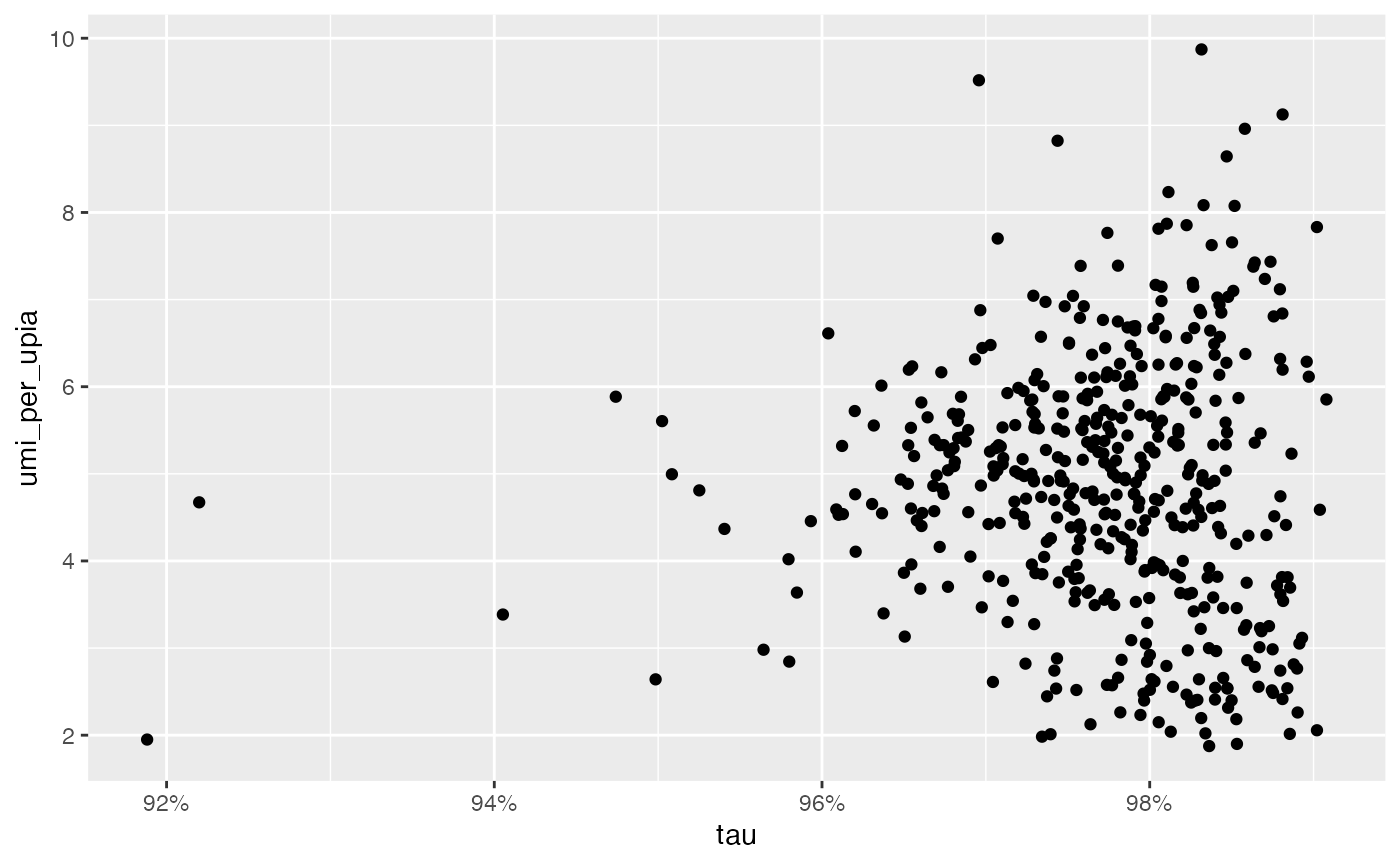
Edge lists, graphs and PXL files
The edge list represents the raw MPX data where each row corresponds to an edge formed between a UPIA and a UPIB pixel. This information is rarely needed for analysis, but is required if we want to load and explore component graphs.
ReadMPX_Seurat doesn’t load the edge list in memory,
instead it keeps track of the paths of the PXL file(s) associated with
the data. We can get the path to the PXL file with the
FSMap function:
FSMap(seur_obj[["mpxCells"]])FSMap returns a tibble with the paths to the PXL files
associated with the Seurat object. In this case, there is
only one PXL file. The “id_map” column is a list, where each element
consists of a tibble with component IDs that can be used as a look up
table to map the “current” component IDs with the “original” component
IDs. If we unnest the “id_map” column, we can see the current and
original component IDs:
## # A tibble: 477 × 4
##    current_id    original_id   sample pxl_file
##    <chr>         <chr>          <int> <chr>
##  1 RCVCMP0000000 RCVCMP0000000      1 PBMC_data/Sample01_human_pbmcs_unstimulat…
##  2 RCVCMP0000002 RCVCMP0000002      1 PBMC_data/Sample01_human_pbmcs_unstimulat…
##  3 RCVCMP0000003 RCVCMP0000003      1 PBMC_data/Sample01_human_pbmcs_unstimulat…
##  4 RCVCMP0000005 RCVCMP0000005      1 PBMC_data/Sample01_human_pbmcs_unstimulat…
##  5 RCVCMP0000006 RCVCMP0000006      1 PBMC_data/Sample01_human_pbmcs_unstimulat…
##  6 RCVCMP0000007 RCVCMP0000007      1 PBMC_data/Sample01_human_pbmcs_unstimulat…
##  7 RCVCMP0000008 RCVCMP0000008      1 PBMC_data/Sample01_human_pbmcs_unstimulat…
##  8 RCVCMP0000010 RCVCMP0000010      1 PBMC_data/Sample01_human_pbmcs_unstimulat…
##  9 RCVCMP0000012 RCVCMP0000012      1 PBMC_data/Sample01_human_pbmcs_unstimulat…
## 10 RCVCMP0000013 RCVCMP0000013      1 PBMC_data/Sample01_human_pbmcs_unstimulat…
## # ℹ 467 more rows
If we were to rename the component IDs of the Seurat object, the “current_id” column will be updated, but the “original_id” column will remain unchanged:
seur_obj_renamed <- RenameCells(seur_obj, new.names = paste0("A_", colnames(seur_obj)))

FSMap(seur_obj_renamed[["mpxCells"]]) %>%
  tidyr::unnest(id_map)
## # A tibble: 477 × 4
## current_id original_id sample pxl_file
## <chr> <chr> <int> <chr>
## 1 A_RCVCMP0000000 RCVCMP0000000 1 PBMC_data/Sample01_human_pbmcs_unstimul…
## 2 A_RCVCMP0000002 RCVCMP0000002 1 PBMC_data/Sample01_human_pbmcs_unstimul…
## 3 A_RCVCMP0000003 RCVCMP0000003 1 PBMC_data/Sample01_human_pbmcs_unstimul…
## 4 A_RCVCMP0000005 RCVCMP0000005 1 PBMC_data/Sample01_human_pbmcs_unstimul…
## 5 A_RCVCMP0000006 RCVCMP0000006 1 PBMC_data/Sample01_human_pbmcs_unstimul…
## 6 A_RCVCMP0000007 RCVCMP0000007 1 PBMC_data/Sample01_human_pbmcs_unstimul…
## 7 A_RCVCMP0000008 RCVCMP0000008 1 PBMC_data/Sample01_human_pbmcs_unstimul…
## 8 A_RCVCMP0000010 RCVCMP0000010 1 PBMC_data/Sample01_human_pbmcs_unstimul…
## 9 A_RCVCMP0000012 RCVCMP0000012 1 PBMC_data/Sample01_human_pbmcs_unstimul…
## 10 A_RCVCMP0000013 RCVCMP0000013 1 PBMC_data/Sample01_human_pbmcs_unstimul…
## # ℹ 467 more rowsThe current IDs will always be unique, but the original IDs are often duplicated as components follow the same naming convention across data sets. The table above helps us to map the current IDs to the correct original IDs and PXL file(s).
If we need to load MPX component graphs in memory, we can use the
LoadCellGraphs function. Under the hood,
LoadCellGraphs uses the table above to sort out where the
edge list data is stored, reads the edge list data and converts it to a
graph object per component.
For example, we can load the graphs for two selected components like this:
seur_obj <- LoadCellGraphs(seur_obj, cells = c("RCVCMP0000228", "RCVCMP0000231"))We can then fetch the loaded CellGraph objects for our
two components using:
CellGraphs(seur_obj)[c("RCVCMP0000228", "RCVCMP0000231")]## $RCVCMP0000228
## A CellGraph object containing a bipartite graph with 3914 nodes and 8022 edges
## Number of markers: 78
##
## $RCVCMP0000231
## A CellGraph object containing a bipartite graph with 4300 nodes and 8027 edges
## Number of markers: 75NOTE: If the PXL file path is invalid, e.g. if the file is missing or
has been moved, LoadCellGraphs will throw an error.